Learn bodybuildr: from one block to a full report

This tutorial starts with a single word on a page and ends with a multi-page PDF report that has a header, a footer, tables, plots, a theme and a block you write yourself. Each step adds one idea, explains what it does and why, and shows the result.

You can read this as a web page, or run the companion script tutorial/learn-bodybuildr.R line by line in Positron or RStudio. The script has the same code, with this text as comments.

Contents

Work through the parts in order the first time; each one builds on the last. Later, jump straight to the part you need. Every part ends with links to the previous part, this list, and the next part.

Part	What you’ll learn
Part 0: Getting set up	Load the packages and a small helper for looking at your work
Part 1: Your first block	What a block is, how it measures itself, flexible blocks, as_block()
Part 2: Putting blocks together	bb_stack(), bb_cols(), column widths, alignment, nesting
Part 3: Making text look right	Text roles, text_style(), span() and link(), Markdown and HTML
Part 4: Boxes, fills and spacing	bb_box(), line_style(), gradients and stripes, the three kinds of spacing
Part 5: Tables	bb_table(), cell(), table styles, data frames, sync_rows
Part 6: Status marks, dots and legends	bb_status(), bb_dot(), bb_legend()
Part 7: Plots, images and grobs	ggplots, fixed vs flexible heights, bb_image(), bb_grob()
Part 8: Pages	bb_page(), page_template(), headers, footers, tokens, banners, page_layout()
Part 9: Documents	bb_document(), optional pages, page-aware headers, export_pdf()
Part 10: Themes	bb_theme(), custom colours and roles, three ways to apply a theme
Part 11: Writing your own block	new_block(), drawing with the theme, using your block anywhere
Part 12: Debugging layouts	export_pdf(debug = TRUE)
Cheat sheet	Which function to reach for, by task

Part 0: Getting set up

library(bodybuildr)   # the package itself
library(ggplot2)      # only used for the plots in Part 7
library(grid)         # only used for the custom blocks in Part 11
set.seed(1)           # so the "random" data is the same every time

A little helper to see things

bodybuildr only produces PDFs, so you need a quick way to look at a block while you learn. The helper below takes any block, puts it on a page that is exactly as tall as the block, and exports it to PDF:

• When you run the script, the PDF goes into a folder called bodybuildr-tutorial/ in your working directory, and the helper prints its path so you can open it.
• When the vignette is built, the helper also turns the PDF into a picture so it shows up on this page.

You don’t need to understand the helper yet. By the end of Part 8 every line in it will make sense.

preview_dir <- if (isTRUE(getOption("knitr.in.progress"))) {
  file.path(tempdir(), "bodybuildr-tutorial")   # building the vignette: keep files out of the way
} else {
  "bodybuildr-tutorial"                         # running the script: next to you
}
dir.create(preview_dir, showWarnings = FALSE)
.preview_n <- 0

preview <- function(x, width = 6, height = NULL, theme = NULL) {
  .preview_n <<- .preview_n + 1
  file <- file.path(preview_dir, sprintf("step-%02d.pdf", .preview_n))

  if (inherits(x, c("bb_page", "bb_document"))) {
    # A finished page or document: export it as it is.
    export_pdf(x, file)
  } else {
    # A loose block: make a page just big enough to hold it.
    margin <- 0.2
    if (is.null(height)) {
      h <- with_theme(theme, as.numeric(measure_block(x, width - 2 * margin)))
      height <- if (is.na(h)) 2.5 else h + 2 * margin   # NA = "flexible", see Part 1
    }
    tpl <- page_template(width = width, height = height, margin_x = margin,
                         margin_top = margin, margin_bottom = margin,
                         theme = theme, background = "white")
    export_pdf(bb_page(x, template = tpl), file)
  }

  in_knitr <- isTRUE(getOption("knitr.in.progress"))
  if (!in_knitr || !requireNamespace("pdftools", quietly = TRUE)) {
    message("Wrote ", file)
    return(invisible(file))
  }
  n <- pdftools::pdf_info(file)$pages
  pngs <- vapply(seq_len(n), function(i) knitr::fig_path(".png", number = sprintf("%02d-%d", .preview_n, i)),
                 character(1))
  dir.create(dirname(pngs[1]), recursive = TRUE, showWarnings = FALSE)
  pdftools::pdf_convert(file, dpi = 150, filenames = pngs, verbose = FALSE)
  knitr::include_graphics(pngs, dpi = 150)
}

---

Contents  |  Part 1: Your first block →

Part 1: Your first block

1.1 Hello, block

Everything you put on a bodybuildr page is a block. The simplest one is text:

hello <- bb_text("Hello, bodybuildr!")
hello
#> <bb_text>

Printing a block only tells you its type (<bb_text>). A block is a description of something to draw, not a drawing yet. To see it, export it:

preview(hello)

1.2 What makes a block a block: it knows its own height

The one idea behind the whole package: a block can tell you how tall it is once you tell it how wide it may be. measure_block() asks that question:

measure_block(hello, width = 6)
#> [1] 0.125inches

The answer is in inches. All of bodybuildr’s internal lengths are in inches. Wherever a function takes a length you can pass a plain number (inches) or a grid::unit() such as unit(12, "pt") or unit(1, "cm").

For one short line, the height is one line of text. Things get more interesting with a longer paragraph:

paragraph <- bb_text(paste(
  "Text wraps to whatever width it is given. Give it a wide space and it",
  "uses few lines; squeeze it into a narrow column and it becomes taller.",
  "Nobody has to type a height anywhere: the block measures itself."
))

measure_block(paragraph, width = 6)   # wide: few lines
#> [1] 0.305572851805729inches
measure_block(paragraph, width = 2)   # narrow: more lines, taller
#> [1] 1.20843711083437inches

preview(paragraph, width = 6)

preview(paragraph, width = 2.4)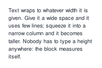

That’s why bodybuildr pages never need hand-tuned row heights. If a translation makes a sentence twice as long, the block gets taller and everything below moves down.

1.3 Flexible blocks: “I’ll take whatever height you give me”

Some blocks have no natural height. An empty space, or a plot, could be any height. bodybuildr calls these flexible blocks, and measure_block() returns NA for them:

measure_block(bb_spacer(), width = 6)        # flexible empty space: NA
#> [1] NAinches
measure_block(bb_spacer(0.5), width = 6)     # fixed empty space: 0.5 in
#> [1] 0.5inches
measure_block(bb_spacer(unit(18, "pt")), 6)  # units work too: 18pt = 0.25 in
#> [1] 0.24906600249066inches

Remember the word flexible. It explains how plots stretch next to tables, how a footer gets pushed down, and much more later on.

1.4 You rarely need to call bb_text() yourself

Anywhere a block is expected, you can pass ordinary R objects. bodybuildr converts them with as_block():

You pass	It becomes
a string or number	bb_text()
a ggplot	bb_plot()
a grid grob	bb_grob()
a path to a .png/.jpg, or an image array	bb_image()
NULL	nothing (it’s skipped)

class(as_block("just a string"))
#> [1] "bb_text"  "bb_block"
class(as_block(42))
#> [1] "bb_text"  "bb_block"
as_block(NULL)
#> NULL

So bb_stack("a", "b") (next part) is the same as bb_stack(bb_text("a"), bb_text("b")).

---

← Part 0  |  Contents  |  Part 2: Putting blocks together →

Part 2: Putting blocks together

A page is a few blocks arranged in two directions: top to bottom (bb_stack()) and side by side (bb_cols()). Those two functions, nested inside each other, can build almost any layout.

2.1 Stacking blocks vertically

stack <- bb_stack(
  "First line.",
  "Second line.",
  "Third line."
)
preview(stack)

The blocks touch. Use gap to add space between them:

preview(bb_stack("First line.", "Second line.", "Third line.", gap = 0.15))

gap can also hold one value per pair of neighbours. With three blocks there are two gaps:

preview(bb_stack("Title", "Right under the title", "Far below", gap = c(0.02, 0.4)))

A stack’s height is the heights of its children plus the gaps, so a stack is itself a block that knows its height:

measure_block(bb_stack("a", "b", "c", gap = 0.15), width = 6)
#> [1] 0.675inches

2.2 Placing blocks side by side

bb_cols() splits the available width into columns, one per block:

left_text <- bb_text(paste(rep("This column has a lot to say.", 6), collapse = " "))
right_text <- bb_text("This one doesn't.")

preview(bb_cols(left_text, right_text, gap = 0.3))

How it works:

1. The row gets a width (here, the 5.6 in inside the preview page).
2. It takes off the gap and splits the rest into equal columns.
3. It asks each child how tall it is at its column width.
4. The row is as tall as its tallest child.

The width goes down and the heights come back up. That’s the whole layout algorithm.

2.3 Choosing column widths

There are three ways to set widths:

# 1. NULL (the default): equal columns
equal <- bb_cols(left_text, right_text, gap = 0.3)

# 2. Numbers: proportions. c(2, 1) means "the first is twice as wide".
proportional <- bb_cols(left_text, right_text, widths = c(2, 1), gap = 0.3)

# 3. Units: mix fixed and proportional widths. "null" means "share what's
#    left". Here the right column is exactly 1.5 in and the left gets the rest.
mixed <- bb_cols(left_text, right_text, gap = 0.3,
                 widths = unit(c(1, 1.5), c("null", "in")))

preview(bb_stack(equal, proportional, mixed, gap = 0.3))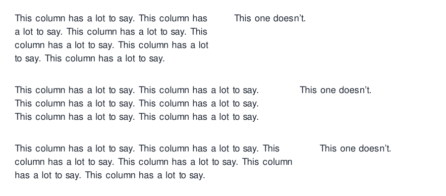

2.4 Vertical alignment and empty columns

By default, shorter columns sit at the top of the row. valign changes that:

preview(bb_cols(left_text, right_text, widths = c(2, 1), gap = 0.3, valign = "center"))

Passing NULL leaves a column empty, which is handy for keeping alignment across several rows:

preview(bb_cols("one", NULL, "three"))

2.5 Nesting: the real power

Since bb_stack() and bb_cols() both return blocks, you can put one inside the other as deep as you like:

nested <- bb_cols(
  bb_stack(
    bb_text("A heading", style = "subheading"),
    bb_text(paste(rep("Some body text under the heading.", 4), collapse = " ")),
    gap = 0.05
  ),
  bb_stack("Point A", "Point B", "Point C", gap = 0.05),
  widths = c(3, 1), gap = 0.3
)
preview(nested)

---

← Part 1  |  Contents  |  Part 3: Making text look right →

Part 3: Making text look right

3.1 Text roles

You’ve already seen style = "subheading". bodybuildr’s theme defines a set of named text roles: a size, weight and colour for each kind of text. Pass the name of a role as style:

roles <- c("body", "note", "small", "subheading", "section", "refs", "legend", "footer")
preview(bb_stack(.list = lapply(roles, function(r) bb_text(paste("This is the", r, "role"), style = r)),
                 gap = 0.06))

(.list = lets you hand a stack a list of blocks instead of typing them out one by one.)

Roles mean you decide what kind of text something is, and the theme decides how that kind looks. Change the theme and every note on every page changes with it (Part 10).

3.2 text_style(): change only what you need

When a role isn’t quite right, use text_style(). It lists only the properties you want to change. Everything else is inherited:

preview(bb_stack(
  # inherits from body text, changes weight and colour
  bb_text("Body text, but bold and muted", style = text_style(weight = 700, color = "muted")),
  # the first argument is a role to start from
  bb_text("Start from 'small', make it italic", style = text_style("small", italic = TRUE)),
  # letter case
  bb_text("make me shout", style = text_style(case = "upper")),
  # size in points, line height as a multiple of the size
  bb_text("Big and airy", style = text_style(size = 16, lineheight = 1.6)),
  gap = 0.1
))

The properties are size, weight (100 to 900, or names like "semibold"), color, family, italic, lineheight and case.

Colours can be any R colour ("red", "#1E5631") or the name of a theme colour such as "primary", "accent", "muted", "faint", "panel" or "rule_light". Theme names are looked up when the page is drawn, so the same block can be drawn with different themes.

3.3 Styling part of a sentence: span() and link()

span() styles a piece of text inside a longer string. It returns a string, so you build sentences with paste0():

sentence <- paste0(
  "Coverage ", span("rose by 12%", weight = 700, color = "accent"),
  " this year (", span("provisional", italic = TRUE, color = "muted"), ")."
)
preview(bb_text(sentence))

link() marks a URL. In plain text it is underlined, and PDF viewers make it clickable:

preview(bb_text(paste0("Data source: ", link("https://example.org/data"))))

3.4 Plain text, Markdown and HTML

By default, text is plain: what you type is what gets printed. Characters that mean something in Markdown, like *, < or [1], are printed as they are. A newline (\n) starts a new line.

preview(bb_text("Plain: values <80% get a *star* [1].\nSecond line."))

Set markup = "markdown" for bold, italics, bullet lists and headings:

md <- "**Bold**, *italic*, and a list:

- first point
- second point"
preview(bb_text(md, markup = "markdown"))

Or markup = "html" for a small HTML subset (<b>, <i>, <sup>, <sub>, <br>, <span style>):

preview(bb_text("H<sub>2</sub>O and E = mc<sup>2</sup>", markup = "html"))

3.5 Alignment

preview(bb_stack(bb_text("Left (default)"),
                 bb_text("Centred", align = "center"),
                 bb_text("Right", align = "right")))

3.6 Measuring text width

Sometimes you need to know how wide a string will be, for example to size a column to fit a label. text_width() tells you:

text_width("How wide am I?")
#> [1] 0.888888888888889inches
text_width("How wide am I?", style = text_style(size = 18, weight = 700))
#> [1] 1.875inches

---

← Part 2  |  Contents  |  Part 4: Boxes, fills and spacing →

Part 4: Boxes, fills and spacing

4.1 Putting a box around something

bb_box() wraps any block in a box. The look comes from box_style():

preview(bb_box(
  "I'm in a box.",
  box_style(fill = "panel", border = "rule_strong", padding = 0.12, radius = 0.06)
))

• fill: background colour (theme names allowed)
• border: a colour, or a line_style() for width and dash pattern
• padding: space between the border and the content
• radius: rounded corners
• margin: space outside the border

box_style_panel() is a ready-made flat grey panel for notes:

preview(bb_box(bb_text("A flat grey note panel.", style = "note"), box_style_panel()))

4.2 Lines

line_style() describes any line: borders, rules under headers, table dividers. lwd is the line width and lty the dash pattern ("22" means 2 on, 2 off):

preview(bb_box("Dashed accent border",
               box_style(border = line_style("accent", lwd = 1.5, lty = "22"), padding = 0.12)))

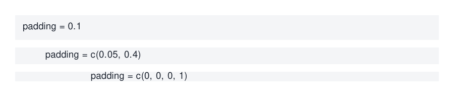
4.3 Padding with 1, 2 or 4 values

Padding and margin work like CSS: one value for all sides, two for (vertical, horizontal), four for (top, right, bottom, left):

preview(bb_stack(
  bb_box("padding = 0.1", box_style(fill = "panel", padding = 0.1)),
  bb_box("padding = c(0.05, 0.4)", box_style(fill = "panel", padding = c(0.05, 0.4))),
  bb_box("padding = c(0, 0, 0, 1)", box_style(fill = "panel", padding = c(0, 0, 0, 1))),
  gap = 0.1
))

4.4 Fancy fills

Besides plain colours, a fill can be a gradient or diagonal stripes:

preview(bb_cols(
  bb_box(bb_text("Gradient", style = text_style(color = "white", weight = 700)),
         box_style(fill = gradient_fill(c("primary", "accent"), dir = "lr"), padding = 0.25)),
  bb_box("Stripes", box_style(fill = stripe_fill(c("panel", "panel_alt"), angle = 45), padding = 0.25)),
  gap = 0.2
))

4.5 A trick: a box around a flexible block is flexible too

Wrap a flexible bb_spacer() in a filled box and you get a coloured bar with no height of its own. Put it in a row and it stretches to the height of its neighbour, which makes a neat accent bar for a quote:

quote_text <- bb_text(paste(rep("A long quotation that wraps over several lines.", 4), collapse = " "),
                      style = text_style(italic = TRUE))
preview(bb_cols(
  bb_box(bb_spacer(), box_style(fill = "accent")),
  quote_text,
  widths = unit(c(0.06, 1), c("in", "null")), gap = 0.15
))

4.6 The three kinds of spacing (and why they’re kept apart)

bodybuildr keeps three kinds of spacing separate so they never interfere:

1. Page margins: the white border around the page. Set once in page_template() (Part 8).
2. Layout gaps: space between blocks, set with gap in bb_stack(), bb_cols() and bb_page().
3. Box spacing: padding and margin inside box_style().

When something looks too spaced out, ask which of the three it is and change it there. Components never add page-level spacing on their own.

---

← Part 3  |  Contents  |  Part 5: Tables →

Part 5: Tables

5.1 The simplest table

A table is a list of rows, and each row is a list of cells:

simple <- bb_table(list(
  list("Apples", "12"),
  list("Bananas", "7"),
  list("Cherries", "143")
))
preview(simple)

Rows are as tall as their content, so long text wraps and the row grows.

5.2 Header, widths and alignment

fruit <- bb_table(
  list(list("Apples", "12"), list("Bananas", "7"), list("Cherries", "143")),
  header = c("Fruit", "Count"),
  widths = c(3, 1),                  # same rules as bb_cols()
  align  = c("left", "right")        # one per column
)
preview(fruit)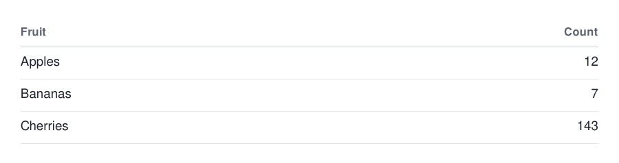

5.3 Styling columns and single cells

col_style styles whole columns. cell() styles one cell:

styled <- bb_table(
  list(
    list("Total population", "45,696,159"),
    list("Surviving infants", "530,193"),
    list("Skilled birth attendance", cell("No data", style = text_style(color = "faint", italic = TRUE))),
    list(cell("of which: urban", style = "small", indent = 0.2), "")
  ),
  header = c("Indicator", "Value"),
  widths = c(2, 1), align = c("left", "right"),
  col_style = list(NULL, text_style(weight = 700))  # NULL = leave column 1 alone
)
preview(styled)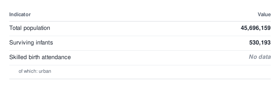

cell() also takes indent (for sub-rows), markup and align.

5.4 Straight from a data frame

Pass a data frame and the column names become the header:

preview(bb_table(head(mtcars[, 1:5], 4), align = "right", header_case = "upper"))

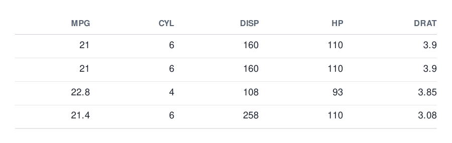
5.5 Two table looks

table_style() (the default) draws only horizontal rules. table_style_grid() is the boxed spreadsheet look. Both take arguments for every detail:

preview(bb_table(head(mtcars[, 1:5], 4), align = "right", style = table_style_grid()))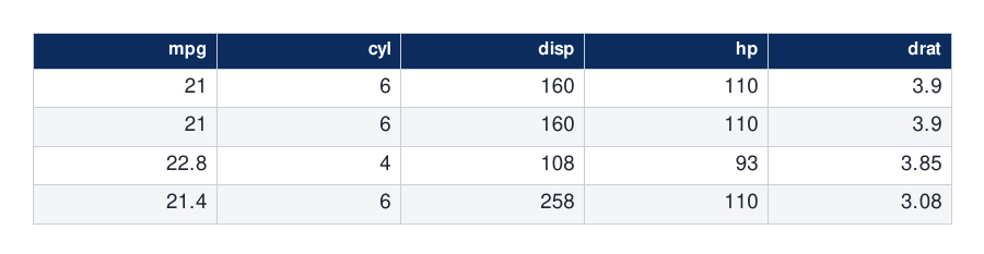

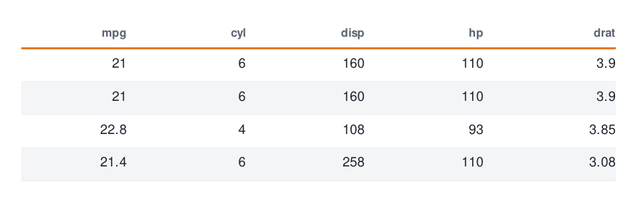
preview(bb_table(
  head(mtcars[, 1:5], 4), align = "right",
  style = table_style(divider = line_style("rule_faint"),       # lighter lines between rows
                      header_rule = line_style("accent", 2),    # thick coloured line under header
                      alt_fill = "panel")                       # zebra stripes
))

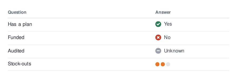
5.6 Any block can be a cell

Cells aren’t limited to text. Anything that is a block works, including the status icons and dots from the next part:

preview(bb_table(
  list(list("Has a plan",   bb_status("yes", label = "Yes")),
       list("Funded",       bb_status("no",  label = "No")),
       list("Audited",      bb_status(NA,    label = "Unknown")),
       list("Stock-outs",   bb_dot(c("accent", "accent", "rule_light")))),
  header = c("Question", "Answer"), widths = c(2, 1)
))

5.7 Lining up two tables side by side

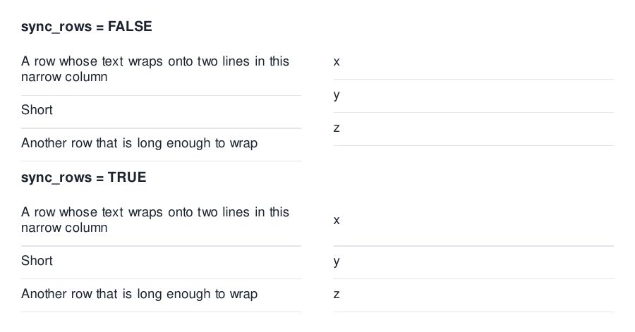
Two tables in a row each size their rows independently, so the dividers don’t line up. sync_rows = TRUE on the row fixes that:

wordy <- bb_table(list(list("A row whose text wraps onto two lines in this narrow column"),
                       list("Short"),
                       list("Another row that is long enough to wrap")))
terse <- bb_table(list(list("x"), list("y"), list("z")))

preview(bb_stack(
  bb_text("sync_rows = FALSE", style = "subheading"),
  bb_cols(wordy, terse, gap = 0.3),
  bb_text("sync_rows = TRUE", style = "subheading"),
  bb_cols(wordy, terse, gap = 0.3, sync_rows = TRUE),
  gap = 0.1
))

---

← Part 4  |  Contents  |  Part 6: Status marks, dots and legends →

Part 6: Status marks, dots and legends

6.1 Status icons

bb_status() draws a filled circle with a check, a cross or a dash. It understands "yes"/"no"/"unknown" and also TRUE/FALSE/NA:

preview(bb_cols(
  bb_status("yes", label = "Meets target"),
  bb_status(FALSE, label = "Below target"),
  bb_status(NA, label = "No data"),
  gap = 0.2
))

The colours come from the theme’s status palette (Part 10).

6.2 Dots and small marks

bb_dot() draws one or more small marks in a row. Colours, shapes and sizes are recycled, so one call can draw a whole pattern:

preview(bb_stack(
  bb_dot("primary"),
  bb_dot(c("accent", "accent", "rule_light", "rule_light")),
  bb_dot("primary", shape = c("circle", "circle", "diamond"), size = c(0.08, 0.08, 0.12)),
  bb_dot(c("#C8503F", "#F2C14E", "#8CC49A"), shape = "square", size = 0.12),
  gap = 0.1
))

6.3 Legends

A legend is a list of legend_key()s. There are six key types: swatch, dot, diamond, status, line and dash.

legend <- bb_legend(
  list(
    legend_key("swatch",  "Below 80%",  "#C8503F"),
    legend_key("swatch",  "80-94%",     "#F2C14E"),
    legend_key("swatch",  "95% +",      "#8CC49A"),
    legend_key("dot",     "Stock-out",  "accent"),
    legend_key("line",    "Trend",      "primary"),
    legend_key("dash",    "Target",     "muted"),
    legend_key("status",  "Meets",      state = "yes")
  ),
  note = "National level"
)
preview(legend)

Legends wrap onto more lines when they run out of room, so they are blocks whose height depends on their width:

measure_block(legend, 7)
#> [1] 0.21875inches
measure_block(legend, 2.5)
#> [1] 0.875inches
preview(legend, width = 2.9)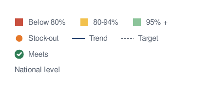

---

← Part 5  |  Contents  |  Part 7: Plots, images and grobs →

Part 7: Plots, images and grobs

7.1 A ggplot is a flexible block

Pass a ggplot anywhere a block goes. Without a height, a plot is flexible: it has no height of its own and takes the height it is given. In a row next to text, that means the height of the text:

p <- ggplot(data.frame(x = 1:30, y = cumsum(rnorm(30))), aes(x, y)) +
  geom_line(colour = "#0C2C5E") +
  theme_minimal()

explanation <- bb_stack(
  bb_text("What happened", style = "subheading"),
  bb_text(paste(rep("The plot on the left is exactly as tall as this column.", 5), collapse = " "),
          style = "note"),
  gap = 0.05
)
preview(bb_cols(p, explanation, widths = c(2, 1), gap = 0.3))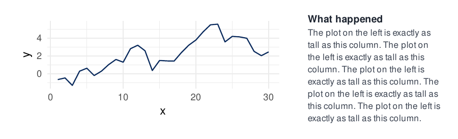

Make the text longer and the plot grows to match.

7.2 Fixed and minimum heights

fixed_plot  <- bb_plot(p, height = 1.2)            # always 1.2 in
min_plot    <- bb_plot(p, min_height = 1.5)        # flexible, never below 1.5 in
fixed_other <- bb_fixed(p, height = 0.8)           # bb_fixed() works on ANY block

measure_block(fixed_plot, 6)
#> [1] 1.2inches
measure_block(min_plot, 6)    # still NA: flexible
#> [1] NAinches
preview(bb_stack(fixed_plot, fixed_other, gap = 0.2))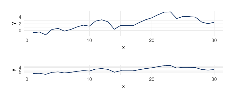

7.3 Images

bb_image() takes a .png/.jpg path, or a numeric array (rows × columns × colour channels). Without a height, an image keeps its natural aspect ratio at the width it gets:

# a small gradient image built from numbers, so this works without any file
img <- array(c(outer(1:60, 1:120, function(i, j) (i + j) / 180),
               outer(1:60, 1:120, function(i, j) j / 120),
               matrix(0.6, 60, 120)), dim = c(60, 120, 3))

preview(bb_cols(
  bb_image(img),                                  # full column width, natural height
  bb_image(img, height = 0.4, align = "left"),    # fixed height, narrower than its slot
  gap = 0.3
))

7.4 Any grid drawing

bb_grob() wraps any grid grob. Give it a height, or leave it flexible:

preview(bb_grob(circleGrob(r = 0.4, gp = gpar(fill = "#E5782A", col = NA)), height = 0.6))

---

← Part 6  |  Contents  |  Part 8: Pages →

Part 8: Pages

So far every preview has been a loose block on a page cut to fit. Real reports use real pages.

8.1 Your first page

bb_page() stacks blocks from the top of the page down. Like bb_stack(), it takes gap:

first_page <- bb_page(
  bb_section_header("My first page"),
  paragraph,
  nested,
  gap = 0.2
)
preview(first_page)

By default a page is US Letter (8.5 × 11 in) with half-inch margins.

8.2 Section headers

bb_section_header() is a title with a small accent marker and a rule underneath. refs adds muted references, and section_header_style() changes everything else:

preview(bb_stack(
  bb_section_header("Default section header", refs = "[1][2]"),
  bb_section_header("No marker, thicker accent rule",
                    style = section_header_style(marker_color = NA, rule = line_style("accent", 2))),
  gap = 0.15
))

8.3 Page templates: size, margins, header and footer

Most reports repeat the same page setup on every page. page_template() holds it once:

template <- page_template(
  width = 8.5, height = 11,              # page size in inches
  margin_x = 0.6,                        # left & right margins
  margin_top = 0.5, margin_bottom = 0.4,
  header = bb_running_header("Field Report", "{region}"),
  footer = bb_page_footer("My Organisation, 2026", "{region} · page {page} of {pages}"),
  header_gap = 0.25                      # space between header and body
)

page_north <- bb_page(
  bb_section_header("Notes from the North"),
  paragraph,
  styled,
  template = template,
  gap = 0.2,
  data = list(region = "North")          # fills {region}
)
preview(page_north)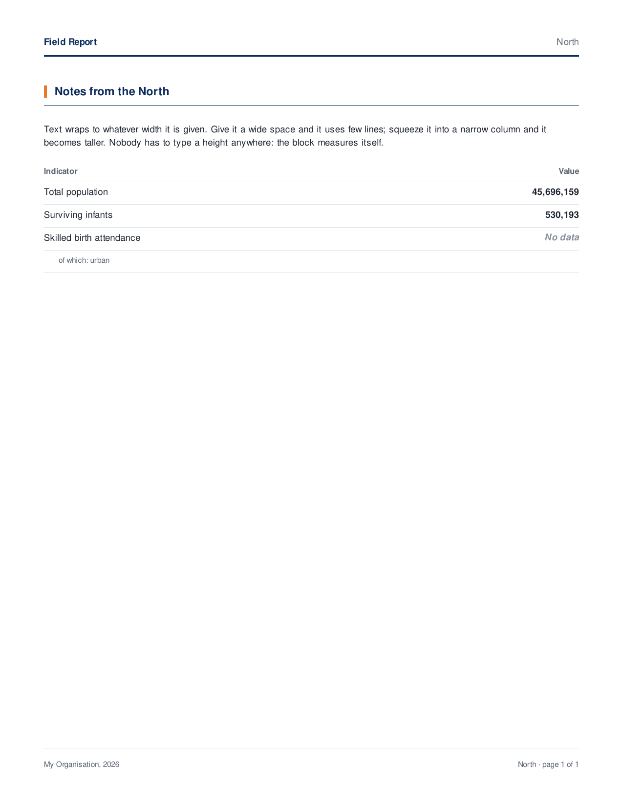

What to notice:

• {region}, {page} and {pages} are tokens. {page} and {pages} are filled in at export time. Anything else comes from the page’s data. So one template serves every page.
• The footer is pinned to the bottom margin. However little content there is, the footer stays in the same place on every page.
• The body runs between the header and the footer.

8.4 Filling the page: flexible blocks again

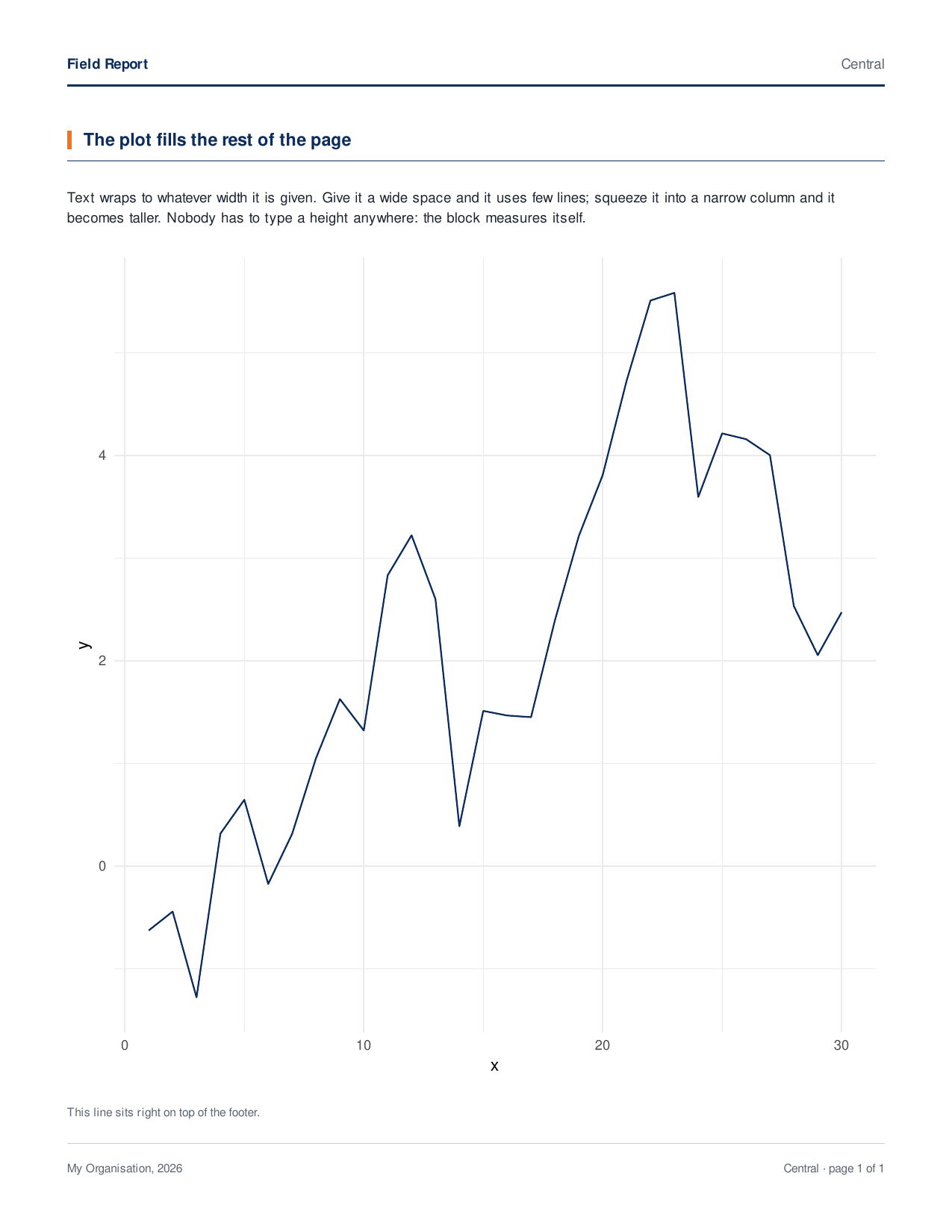
A flexible block in a page body gets all the height that’s left over. A plain bb_spacer() pushes everything after it to the bottom, and a plot with no height fills the gap:

preview(bb_page(
  bb_section_header("The plot fills the rest of the page"),
  paragraph,
  p,                                       # flexible: takes all the leftover height
  bb_text("This line sits right on top of the footer.", style = "small"),
  template = template, gap = 0.2, data = list(region = "Central")
))

8.5 How much room is left? And what if it’s too much?

page_layout() measures a page without exporting it:

page_layout(page_north)[c("available", "used", "free")]
#> $available
#> [1] 8.91375
#> 
#> $used
#> [1] 2.626441
#> 
#> $free
#> [1] 6.287309

free is in inches. If it’s negative, the content doesn’t fit, and export_pdf() warns you and says by how much:

too_long <- bb_page(.list = rep(list(paragraph), 40), template = template, data = list(region = "X"))
page_layout(too_long)$free
#> [1] -3.309164

For automated pipelines, bb_page(..., overflow = "error") turns the warning into an error so nothing silently runs off the page.

8.6 Banners and full-bleed blocks

A banner is a coloured band across the full width of the page. It ignores the side margins (it is full bleed). Used as a page header, it sits flush with the top edge:

banner_page <- bb_page(
  bb_section_header("A page with a banner"),
  paragraph,
  # any block can be full bleed when it's a direct child of a page:
  bb_full_bleed(bb_box(bb_text("Full-bleed band", style = text_style(color = "white")),
                       # 0.6 in side padding lines the text up with the page margin
                       box_style(fill = "accent", padding = c(0.12, 0.6)))),
  template = template,
  header = bb_banner("Annual Report", "North region, 2026"),   # overrides the template header
  gap = 0.2, data = list(region = "North")
)
preview(banner_page)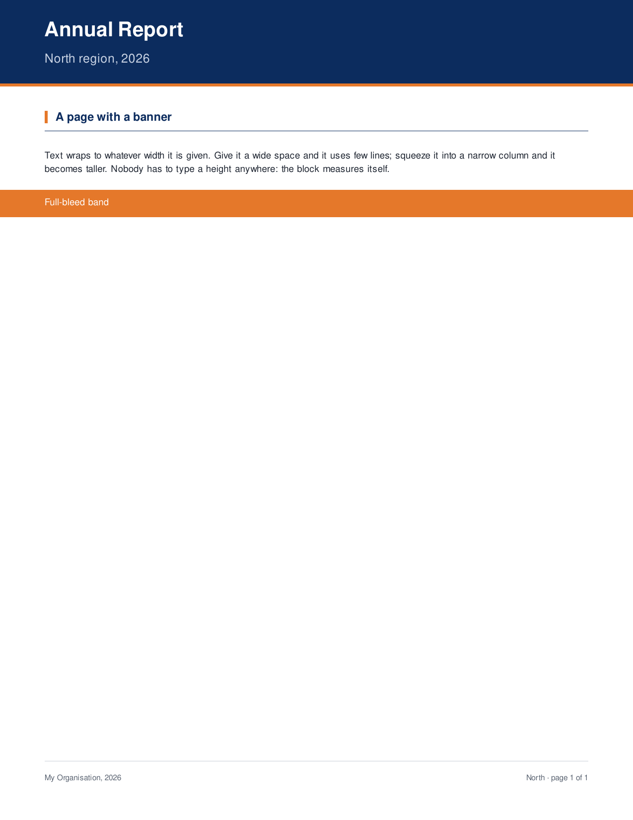

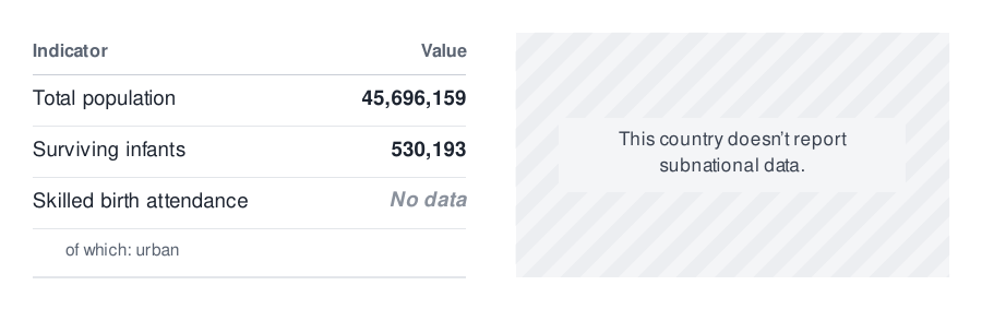
8.7 Placeholders for missing content

When a data source doesn’t provide something, bb_placeholder() fills the space with a patterned panel and a sentence. It is flexible, so in a row it takes the height of its neighbour:

preview(bb_cols(
  styled,
  bb_placeholder("This country doesn't report subnational data."),
  gap = 0.3
))

---

← Part 7  |  Contents  |  Part 9: Documents →

Part 9: Documents

9.1 Several pages in one PDF

bb_document() collects pages. export_pdf() writes them into one file and numbers them:

page_south <- bb_page(bb_section_header("Notes from the South"), paragraph, fruit,
                      template = template, gap = 0.2, data = list(region = "South"))

doc <- bb_document(page_north, page_south)
preview(doc)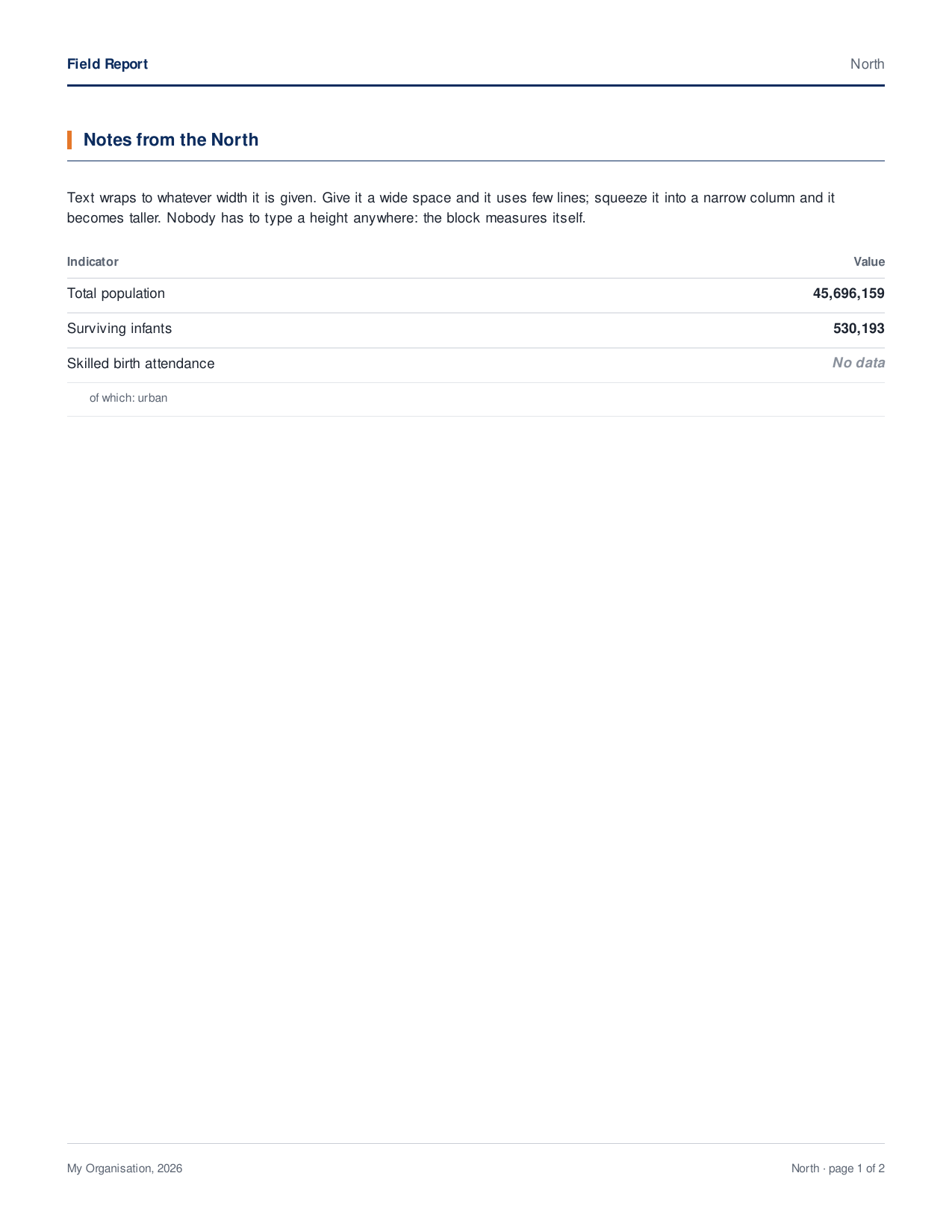

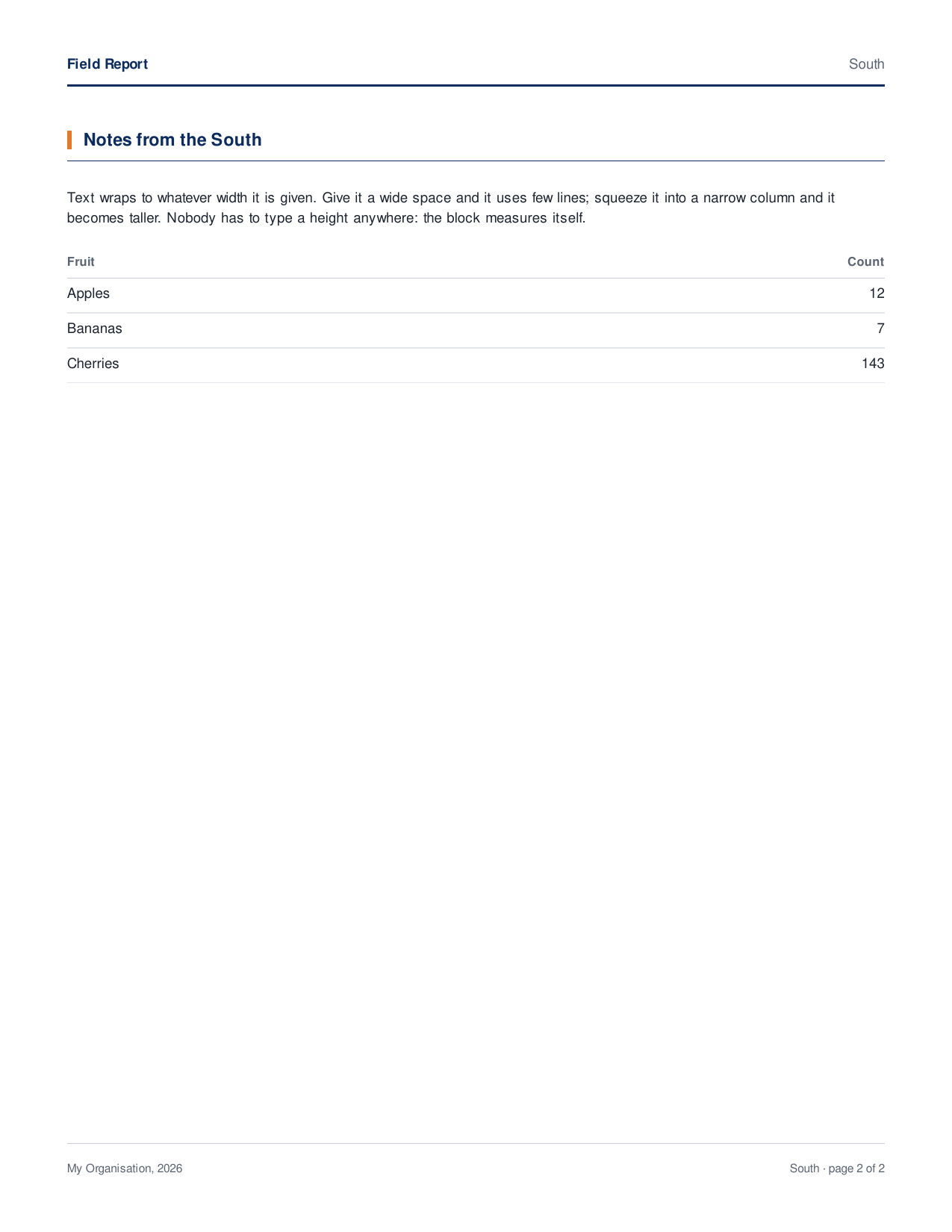
Look at the footers: “page 1 of 2”, “page 2 of 2”.

9.2 Optional pages

NULL pages are dropped before numbering. So you can build a page only when there’s data for it, and the “page X of Y” numbers stay right:

have_east_data <- FALSE
page_east <- if (have_east_data) bb_page("East", template = template) else NULL

doc <- bb_document(page_north, page_east, page_south)   # still 2 pages
length(doc$pages)
#> [1] 2

9.3 Headers that depend on the page

A template’s header or footer can be a function that gets the page context (ctx$page, ctx$pages, ctx$data) and returns a block. That’s how you get a banner on the cover and a running header on later pages:

smart_template <- page_template(
  header = function(ctx) {
    if (ctx$page == 1) bb_banner("Annual Report", "Cover page")
    else bb_running_header("Annual Report", "page {page}")
  },
  footer = bb_page_footer("My Organisation", "{page} / {pages}")
)
preview(bb_document(
  bb_page(bb_section_header("Introduction"), paragraph, template = smart_template),
  bb_page(bb_section_header("Details"), paragraph, template = smart_template)
))

9.4 Exporting

export_pdf(doc, "my-report.pdf")

export_pdf() uses the Cairo PDF device when available, for full Unicode and proper font weights. Every page in one export must have the same size.

---

← Part 8  |  Contents  |  Part 10: Themes →

Part 10: Themes

10.1 What a theme holds

A theme has three things:

• a palette: named colours (primary, accent, muted, panel, rule_light, …)
• text roles: the body, note, section, … styles from Part 3
• a status palette: the yes/no/unknown colours of bb_status()

bb_get_theme()
#> <bb_theme> font: sans  base size: 9 pt
#> colours: primary, accent, ink, text2, muted, faint, rule_strong, rule_light, rule_faint, panel, panel_alt, on_primary, on_primary_muted 
#> text roles: body, table_body, note, small, subheading, section, refs, title, subtitle, running, running_right, table_header, legend, footer, status_label, placeholder

10.2 Making your own theme

bb_theme() only needs what you want to change. Here’s a green, serif theme with one new colour (moss) and one new text role (callout):

forest <- bb_theme(
  font = "serif",
  base_size = 10,                          # body text size in points; all roles scale with it
  colors = list(primary = "#1E5631", accent = "#C1A35F", panel = "#EEF3EC",
                moss = "#4C7A34"),         # a brand-new colour name
  text = list(
    section = text_style(italic = TRUE, weight = 400),               # change an existing role
    callout = text_style(size = 13, weight = 700, color = "moss")    # a brand-new role
  ),
  status = c(yes = "#4C7A34", no = "#A23B2A", unknown = "#9AA1AA")
)

10.3 Same blocks, different theme

None of these blocks names a colour directly. They all use role and palette names, so a theme can restyle them:

themed_blocks <- bb_stack(
  bb_section_header("A themed section"),
  bb_text("Body text in the theme's font.", style = "body"),
  bb_box(bb_text("A panel in the theme's panel colour.", style = "note"), box_style_panel()),
  bb_status("yes", label = "Status colour from the theme"),
  legend,
  gap = 0.12
)
preview(themed_blocks)                   # default theme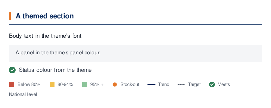

preview(themed_blocks, theme = forest)   # forest theme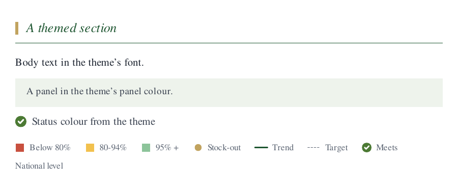

10.4 Three ways to apply a theme

# 1. On a page template: the theme applies while those pages are exported.
#    This is the recommended way.
page_template(theme = forest)

# 2. Temporarily, for one expression:
with_theme(forest, measure_block(themed_blocks, 6))

# 3. Globally, for everything afterwards:
old <- bb_set_theme(forest)
bb_set_theme(old)                        # put the previous one back

One caveat: a custom role like callout only exists in the theme that defines it. A block that uses style = "callout" will fail with an “Unknown text role” error under any other theme.

---

← Part 9  |  Contents  |  Part 11: Writing your own block →

Part 11: Writing your own block

When nothing built in draws what you need, write a block. A block needs just two functions:

• measure(width): “how tall are you at this width?” Return inches, or NA to be flexible.
• render(width, height): “draw yourself.” Return a grid grob. It’s drawn in a box exactly width × height inches. Inside that box, grid’s "npc" units run from 0 (left/bottom) to 1 (right/top).

11.1 The simplest possible block: a coloured bar

bar <- new_block(
  "bar",                                                    # a name for the block type
  measure = function(width) 0.1,                            # always 0.1 in tall
  render  = function(width, height) rectGrob(gp = gpar(fill = "#E5782A", col = NA))
)
preview(bb_stack("Above the bar", bar, "Below the bar", gap = 0.08))

rectGrob() with no arguments fills its whole box, and the box is exactly the size measure() asked for.

11.2 A block that uses the theme

Good blocks don’t hard-code colours or fonts. They read them from the theme at draw time, so they follow theme changes like built-in blocks do:

• bb_get_theme()$colors is the palette.
• text_gpar(style) turns a role name or text_style() into grid’s graphics parameters (font, size, colour).

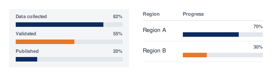
Here’s a labelled progress bar:

progress <- function(label, fraction, color = "primary") {
  label_style <- text_style("small", weight = 700)
  bar_height  <- 0.1
  spacing     <- 0.04

  # One line of text in inches: font size (points) x line height / 72
  line_height <- function() {
    gp <- text_gpar(label_style)
    gp$fontsize * gp$lineheight / 72
  }

  new_block(
    "progress",
    measure = function(width) line_height() + spacing + bar_height,
    render = function(width, height) {
      palette <- bb_get_theme()$colors
      fill    <- palette[[color]] %||% color        # theme name, or a plain colour
      gTree(children = gList(
        # label at the top left, percentage at the top right
        textGrob(label, x = 0, y = 1, just = c("left", "top"), gp = text_gpar(label_style)),
        textGrob(sprintf("%d%%", round(100 * fraction)), x = 1, y = 1,
                 just = c("right", "top"), gp = text_gpar(label_style)),
        # grey track, then the coloured part, both along the bottom
        rectGrob(x = 0, y = 0, width = 1, height = unit(bar_height, "in"),
                 just = c("left", "bottom"), gp = gpar(fill = palette$rule_light, col = NA)),
        rectGrob(x = 0, y = 0, width = fraction, height = unit(bar_height, "in"),
                 just = c("left", "bottom"), gp = gpar(fill = fill, col = NA))
      ))
    }
  )
}

bars <- bb_stack(
  progress("Data collected", 0.82),
  progress("Validated", 0.55, color = "accent"),
  progress("Published", 0.20),
  gap = 0.12
)
measure_block(bars, 3)
#> [1] 1.035inches
preview(bars, width = 3.4)

preview(bars, width = 3.4, theme = forest)   # follows the theme for free

11.3 Custom blocks work everywhere

Your block is a full citizen. It can go in boxes, columns, tables and pages:

preview(bb_cols(
  bb_box(bars, box_style_panel()),
  bb_table(list(list("Region A", progress("", 0.7)),
                list("Region B", progress("", 0.3, "accent"))),
           header = c("Region", "Progress"), widths = c(1, 2)),
  gap = 0.3
))

11.4 Optional extras

new_block() takes a few more optional arguments:

• min_height = function(width): for flexible blocks, the smallest height they can be squeezed to.
• natural_width = function(width): for marks narrower than their slot, the width they actually use. Tables use it to align the mark to the right or centre.
• full_bleed = TRUE: span the full page width when placed directly on a page.

One rule: if you measure text or grobs yourself with grid (for example convertWidth()), wrap it in with_measure_device(). That way measurements use the same kind of device as the export, and no stray Rplots.pdf gets created.

---

← Part 10  |  Contents  |  Part 12: Debugging layouts →

Part 12: Debugging layouts

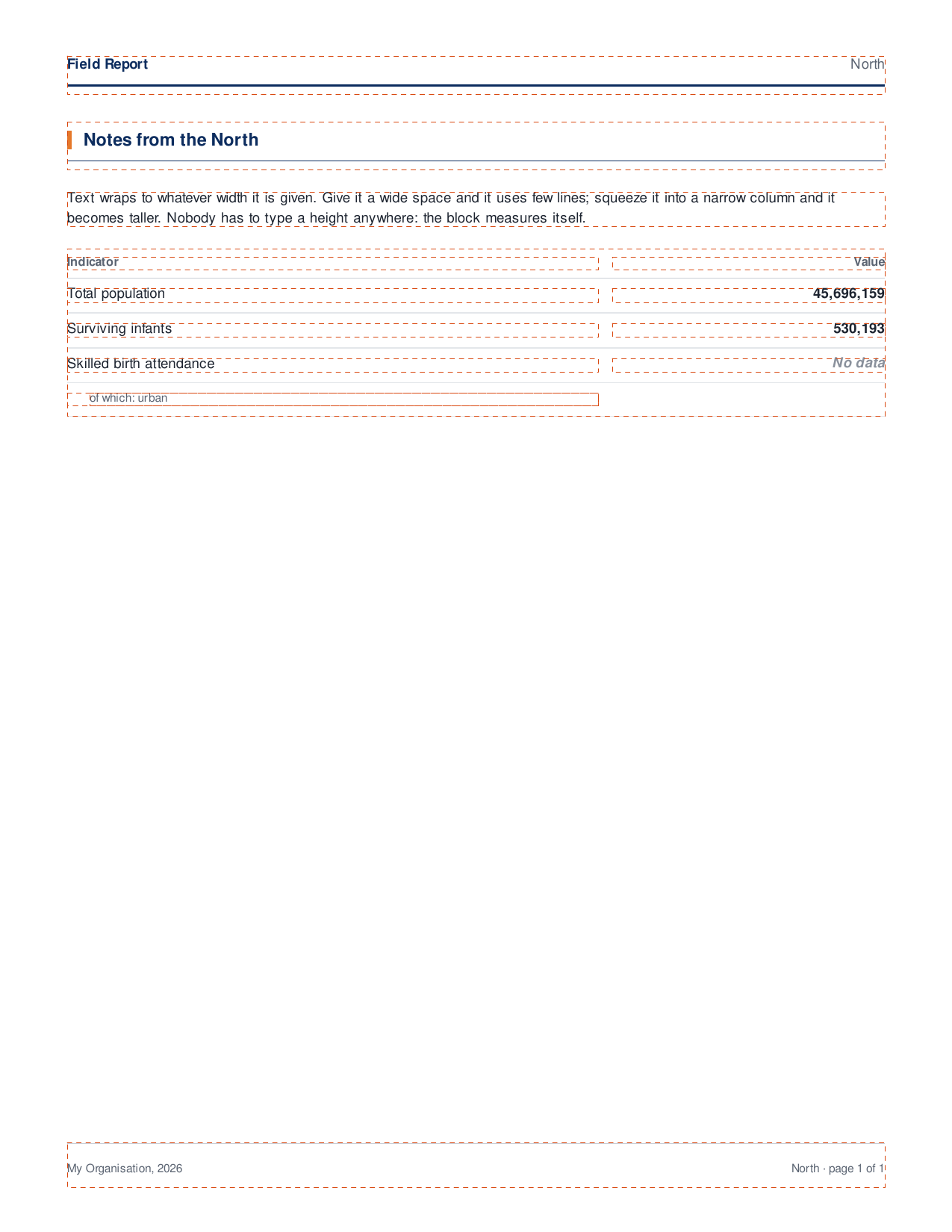
When the spacing looks off, export with debug = TRUE. Every block’s box is outlined with a dashed line, so you can see which gap, padding or margin is causing it:

f <- file.path(preview_dir, "debug.pdf")
export_pdf(page_north, f, debug = TRUE)
if (isTRUE(getOption("knitr.in.progress")) && requireNamespace("pdftools", quietly = TRUE)) {
  png <- knitr::fig_path(".png", number = "debug")
  dir.create(dirname(png), recursive = TRUE, showWarnings = FALSE)
  pdftools::pdf_convert(f, dpi = 150, filenames = png, verbose = FALSE)
  knitr::include_graphics(png, dpi = 150)
}

---

← Part 11  |  Contents  |  Cheat sheet →

Cheat sheet

I want to…	Use
put text on the page	bb_text(), or just a string
style text	style = "role" or text_style(); span()/link() inside a sentence
stack things vertically	bb_stack(..., gap =)
put things side by side	bb_cols(..., widths =, gap =, valign =)
add a box, panel or border	bb_box(x, box_style(...)), box_style_panel()
add empty space	bb_spacer(height); bb_spacer() to fill leftover space
force a height	bb_fixed(x, height)
show a table	bb_table(), cell(), table_style(), table_style_grid()
show yes/no marks	bb_status(), bb_dot()
add a legend	bb_legend(list(legend_key(...)))
show a plot, image or grob	pass it in, or bb_plot() / bb_image() / bb_grob()
title a section	bb_section_header()
a coloured band across the page	bb_banner(), bb_full_bleed()
mark missing content	bb_placeholder()
set up pages	page_template(), bb_page(), bb_document()
check how full a page is	page_layout()
write the PDF	export_pdf(x, file, debug =)
change the whole look	bb_theme() on page_template(theme =)
draw something new	new_block(measure =, render =), text_gpar()

---

← Part 12  |  Contents